I created a tool for the public company "Central Garden & Pet" to choose an optimal price point for its pet products based on past performance, and set up their Nielsen data in an optimal way for making future price predictions. Note, due to confidentiality, certain information is left out of this presentation.
Table of Contents
Background
Central Garden & Pet
Central Garden & Pet (NASDAQ Ticker: CENT) is a leading innovator, marketer, and producer of quality branded pet products to major and independent retailers nationwide.
Nielsen Data
This project analyzes weekly Nielsen retail pricing data for many retailers (including Central Garden & Pet) over the last three years. Nielsen collects this data to create a picture of the total market.
- It includes 80 different price & volume identifiers based on promotional, non-promotional, and average/base prices each week for current and previous year.
- Data focuses on Central Garden & Pet's small animal food business segment, which amounts to approximately 60,000 rows.
- I created price elasticity scores for each price point based on historical price. A price elasticity of 5 means a 1% increase in price leads to a 5% decrease in quantity.
Dataframe Preparation
Imports
# general
import os
import json
import pickle
import numpy as np
import pandas as pd
import statsmodels.formula.api as smf
from IPython.display import Image

# sklearn
from sklearn import metrics
from sklearn import tree
from sklearn.cross_validation import train_test_split
from sklearn.ensemble import RandomForestRegressor
from sklearn.linear_model import LinearRegression
from sklearn.preprocessing import PolynomialFeatures
from sklearn.pipeline import make_pipeline

# graphing
%matplotlib inline
from matplotlib import pyplot as plt
import matplotlib.pyplot as plt
from IPython.core.pylabtools import figsize
import seaborn as sns
from seaborn import plt
import patsy

import warnings
warnings.filterwarnings('ignore')
Read in the data
df = pd.read_csv('petfood_projectkojak.csv')
Function to clean and standardize column names
def clean_names(columns):
    columns = [str(col).lower().replace('[', '').replace(']', '').replace(' ', '_').replace('$', 'usd').replace('%', 'percent_')
               for col in columns]
    return columns

df.columns = clean_names(df.columns)
Creating dummy variable columns for categorical features
Each new dataframe is merged with the previous dataframe.
df_market = pd.get_dummies(df['market'])
df_new = pd.concat([df, df_market], axis=1)

df_size = pd.get_dummies(df_new['base_size'])
df_new0 = pd.concat([df_new, df_size], axis=1)

df_years = pd.get_dummies(df_new0['year'])
df_new1 = pd.concat([df_new0, df_years], axis=1)

df_brand_high = pd.get_dummies(df_new1['brand_high'])
df_new2 = pd.concat([df_new1, df_brand_high], axis=1)

df_target_animal = pd.get_dummies(df_new2['target_animal'])
df_new3 = pd.concat([df_new2, df_target_animal], axis=1)

df_new3.columns = clean_names(df_new3.columns)
df_cgp = df_new3
Optimal Price Point
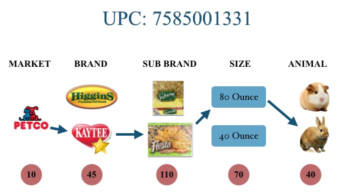
A small animal food product is looked at through its unique UPC code, which takes into account the product's market, brand, sub brand, size, and animal. Central Garden & Pet's small animal food brand is called "Kaytee". Here's a diagram that illustrates a product UPC code. Note, the red circles represent how many unique items there are. For example, there are 110 different sub brands.
Function that finds optimal price point
def find_optimal(df):
    x = np.array(list(df.avg_unit_price))
    y = np.array(list(df.usd))
    x_df = pd.DataFrame(x)
    y_df = pd.DataFrame(y)

    degree = 3 # Set the degree of our polynomial

    # Generate the model type with make_pipeline. First step is to generate
    # degree polynomial features in the input features and then run a linear
    # regression on the resulting features.
    est = make_pipeline(PolynomialFeatures(degree), LinearRegression())
    est.fit(x_df, y_df) # Fit our model to the training data

    range_min = x.mean() - 1*x.std()
    range_max = x.mean() + 1*x.std()
    x0 = np.arange(range_min, range_max, .05, dtype=None)
    x_df0 = pd.DataFrame(x0)
    pred0 = est.predict(x_df0)
    max_index = np.argmax(pred0)

    return x0[max_index]
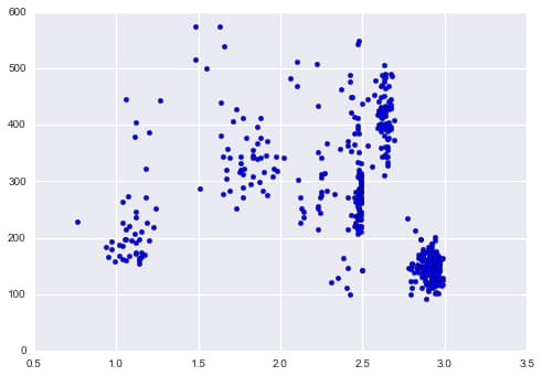
Example of how optimal price function works
df_cgp_petsmart_sku = df_cgp.ix[df_cgp.upc == 2685100451, :]
df_cgp_petsmart_sku = df_cgp.ix[df_cgp.upc == 2685100451, :]
plt.scatter(df_cgp_petsmart_sku.avg_unit_price, df_cgp_petsmart_sku.units)
x = np.array(list(df_cgp_petsmart_sku.avg_unit_price))
y = np.array(list(df_cgp_petsmart_sku.usd))
z = np.polyfit(x, y, 3)
x_df = pd.DataFrame(x)
y_df = pd.DataFrame(y)

# Set up the plot
fig,ax = plt.subplots(1,1)
degree = 3
est = make_pipeline(PolynomialFeatures(degree), LinearRegression())
est.fit(x_df, y_df)

# Plot the results
pred = est.predict(x_df)
plt.scatter(x_df,y_df)
plt.plot(x,pred,'or')

# Sort the data to plot it
x_sorted = sorted(x_df.values.T.tolist()[0])
pred_sorted = [j for (i, j) in sorted(zip(x_df.values.flatten().T.tolist(), pred.flatten().tolist()))]
plt.plot(x_sorted, pred_sorted,'-g')
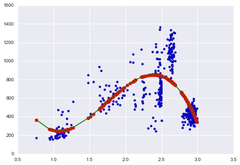
Optimal Price Graph:
- Price vs. Revenue
- Create Range of 1 standard deviation
- Fit third degree polynomial line
- Find optimal point
Implement optimal price function in dataframe
Set new optimal price column filled with zeros:
df_cgp['opt_price'] = pd.Series(np.zeros(len(df_cgp)))
Create product path to filter required data. A UPC code can be the same for different markets and brands, so to filter Central Garden and Pet's Kaytee brand, I create a path filtered also by market and brand_high.
paths = pd.unique(df_cgp[['market', 'brand_high', 'upc']].values)
The code below finds the optimal price for a product and puts it into the new column "opt_price". Works if there are at least 10 data points and if prices don't vary, it gives the average unit price.
threshold = 10
for path in paths:
    df_path = df_cgp[(df_cgp.market == path[0]) & (df_cgp.brand_high == path[1]) & (df_cgp.upc == path[2])]
    num_records = len(df_path)

    if num_records < threshold:
        continue
    if len(df_path.avg_unit_price.unique()) == 1:
        price = df_path.avg_unit_price.iloc[0]
    else:
        price = find_optimal(df_path)

    df_cgp.loc[(df_cgp.market == path[0]) & (df_cgp.brand_high == path[1]) & (df_cgp.upc == path[2]), 'opt_price'] = price
Dataframe Setup for Prediction Analysis
Filtering to Total US Market
df_cgp = df_cgp[df_cgp.market=='Total US Market']
Filtering Total US Market dataframe into two dataframes. One which includes Central Garden & Pet's brand "Kaytee" and the other which includes all other competitor brands.
df_kaytee = df_cgp[df_cgp.brand_high=='KAYTEE']
df_notkaytee = df_cgp[df_cgp.brand_high!='KAYTEE']
Function to convert "week" column into datetime
def convert_weeks(val):
    return val[-8:]

df_kaytee["weeks_dt"] = pd.to_datetime(df_kaytee.loc[:, "weeks"].map(convert_weeks))
df_notkaytee["weeks_dt"] = pd.to_datetime(df_notkaytee.loc[:, "weeks"].map(convert_weeks))
Sort dataframes by week
df_kaytee.sort_values(["market", "upc", "weeks_dt"], inplace=True)
df_notkaytee.sort_values(["market", "upc", "weeks_dt"], inplace=True)
Example code that uses .shift() method to add previous week price data in same row as current week price data. Here's an example of the code on one price category "avg_pe_normal".
The Kaytee Dataframe will now have three new columns: week1_avg_pe_normal, week2_avg_pe_normal, week3_avg_pe_normal.
I do this for every price point and for more than three weeks to get complete picture to analyze.
# avg pe normal
df_kaytee["week1_avg_pe_normal"] = df_kaytee.groupby(["market", "upc"]).avg_pe_normal.shift(1)
df_kaytee["week2_avg_pe_normal"] = df_kaytee.groupby(["market", "upc"]).avg_pe_normal.shift(2)
df_kaytee["week3_avg_pe_normal"] = df_kaytee.groupby(["market", "upc"]).avg_pe_normal.shift(3)
Function to add competitor pricing
This function adds average price for competitor pricing ('competitor_both' column) filtered by market, UPC, and week like above.
def get_competitor_prices(row):
    for week, week_comp_pe in [("week1", "week1_avg_pe_normal_comp"),
                               ("week2", "week2_avg_pe_normal_comp"),
                               ("week3", "week3_avg_pe_normal_comp")]:
        values = [df_notkaytee.loc[(df_notkaytee["weeks"] == row[week])
                     & (df_notkaytee["upc"] == int(comp_upc))
                     & (df_notkaytee["market"] == row["market"]),
                     "avg_pe_normal"].values
        for comp_upc in row["competitor_both"].split(",")]

        values = [val[0] for val in values if len(val) > 0]

        if values:
            row[week_comp_pe] = np.mean(values)
        else:
            row[week_comp_pe] = np.nan

    return row

df_kaytee_comp = df_kaytee.apply(get_competitor_prices, axis="columns")
Conclusion
This project took real-world Nielsen retail data and created a tool for Central Garden & Pet to choose an optimal price for its products based on historical weekly prices and revenue. I then set up the data in an optimal way to make weekly predictions on what prices to set by adding previous week prices as additional columns for each unique price identifier. I similarly did this with competitor prices.
Key accomplishments:
- Price optimization algorithm using polynomial regression to find revenue-maximizing price points across 60,000+ product records
- Feature engineering for time-series prediction by creating lagged price variables for both company and competitor products
- Data pipeline setup that transformed Nielsen retail data into a prediction-ready format with 80+ price and volume features
These additional data points, along with other volume and price feature columns, can then be used with predictive models to set future prices. Due to timing constraints, this project didn't get to include analysis of predictive models on the data, but the foundation has been established for future price prediction work.