This project develops a machine learning model to assess credit risk for loan applicants using a 10,000-record Lending Club dataset. Credit risk remains a fundamental challenge in lending—even approved loans carry default risk, impacting institutional profitability and investor returns.
The objective: predict which loans will default based on borrower characteristics, loan features, and credit history. I tested six ML algorithms, implemented two encoding strategies, and addressed a severe class imbalance (98.5% safe vs 1.5% risky loans).
Key technical challenges tackled:
- Systematic missing value treatment across 54 features
- Class imbalance requiring weighted training
- High-cardinality categorical encoding (state, employment title)
- Model selection optimizing for recall over accuracy
- K-Fold cross-validation and hyperparameter tuning
Results: AdaBoost achieved 0.63 balanced accuracy with 26.4% recall on the risky class—successfully identifying 1 in 4 defaults despite extreme imbalance.
The complete pipeline covers data preprocessing, exploratory analysis, feature engineering, multiple encoding strategies, six ML models, clustering analysis, and business recommendations.
The Problem: Credit Risk in Modern Lending
Every loan carries risk. Even after rigorous credit checks and approval processes, some loans will default—costing financial institutions millions in losses. For peer-to-peer lending platforms like Lending Club, where individual investors bear the risk, accurate credit assessment becomes even more critical.
The challenge is straightforward: Can we predict which approved loans are likely to default?
This project tackles that question using machine learning on a dataset of 10,000 Lending Club loans, building models that identify high-risk borrowers before they miss payments.
Understanding the Data
The analysis began with a comprehensive dataset containing 54 features per loan, including:
- Borrower information: Employment history, income, homeownership status
- Loan characteristics: Amount, interest rate, purpose, term length
- Credit history: Previous delinquencies, credit utilization, account age
- Financial metrics: Debt-to-income ratio, total credit limits
The Challenge: Severe Class Imbalance
The dataset revealed a critical challenge faced by all credit risk models:
- 98.5% of loans were “safe” (Fully Paid or Current)
- Only 1.5% were “risky” (Late payments or in grace period)
This imbalance mirrors reality—most loans don’t default—but it makes prediction difficult. A naive model that simply predicts “safe” for everything would achieve 98.5% accuracy while being completely useless at identifying risk.
The Approach: From Data to Insights
1. Data Preprocessing
Before any modeling could begin, the dataset required careful cleaning:
Missing Value Treatment
- Joint application fields (33% missing) were filled with “N/A” for individual applications
- Delinquency records were marked as “not delinquent” when absent
- Employment information was categorized as “Not Provided” rather than deleted
- A problematic column with no valid data was removed entirely
The key insight: Missing data often carries meaning. A missing employment title might indicate informal work or freelancing—itself a risk signal.
Feature Engineering
- Created binary risk classification (0 = Safe, 1 = Risky)
- Dropped redundant features like sub-grade (kept the more general grade)
- Applied multiple encoding strategies for categorical variables
- Standardized numerical features to prevent scale bias
2. Exploratory Data Analysis: What Makes a Loan Risky?
Initial Findings: Categorical Distribution
The first phase of analysis examined categorical variables through frequency plots:
- California emerged as the most frequent state for loan originations
- 33% of loans had unverified income – a significant risk indicator
- Debt consolidation and credit card payments were the top two loan purposes
- Grade B loans were most frequent in the dataset
- Class imbalance confirmed: “Current” status dominated over “Fully Paid” and delinquent loans
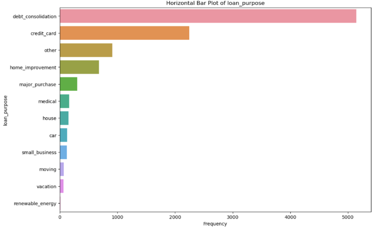 Fig: Distribution of key categorical variables – state, loan purpose, grade, and loan status. Note the severe imbalance with “Current” status dominating the dataset.
Log-Scale Analysis: Uncovering Hidden Patterns
The analysis uncovered several counterintuitive risk patterns using logarithmic scaling:
High-Risk Indicators:
- Missing employment information: Loans without job titles showed elevated default rates
- Long employment tenure: Surprisingly, borrowers with 10+ years at their job had higher risk
- Renter status: Renters defaulted more often than homeowners
- Debt consolidation purpose: These loans carried higher risk than other purposes
- January origination: Loans issued in January showed elevated risk (post-holiday financial strain?)
- Cash disbursement: Non-digital disbursements correlated with higher defaults
The Imbalance Problem in Action:
Using logarithmic scaling revealed patterns invisible in standard visualizations. When 98.5% of loans are safe, linear charts show only the majority class. Log scaling exposed the characteristics of that critical 1.5% risky segment—the loans that actually matter for risk management.
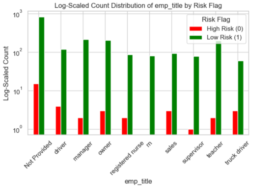
Fig: Log-scale visualization reveals risk patterns in low-frequency categories. Red bars indicate risky loans (Class 1), green bars indicate safe loans (Class 0). Notice how certain categories like “Not Provided” employment and “rent” homeownership show elevated risk ratios.
The Models: Six Approaches to Risk Prediction
Multiple machine learning algorithms were trained and evaluated:
Models Tested:
- Logistic Regression (baseline)
- Random Forest Classifier
- Support Vector Machine (SVM)
- AdaBoost Classifier
- Neural Networks
- LightGBM (gradient boosting)
Handling Class Imbalance
Given the 98.5/1.5 split, all models used computed class weights to ensure the rare risky loans weren’t ignored during training. Without this adjustment, models simply learn to predict “safe” for everything.
Validation Strategy
The analysis employed rigorous validation:
- K-Fold Cross-Validation (5 folds) to ensure robust performance estimates
- GridSearchCV for hyperparameter tuning across multiple models
- Stratified sampling to maintain class balance in train/test splits
Advanced Experimentation
A separate experimental track used target encoding, categorical encoding, and LightGBM with 5-fold stratified cross-validation. This approach generated an exceptional ROC-AUC score of 0.995, demonstrating the model’s strong ability to distinguish between safe and risky loans.
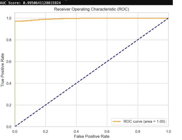 Fig: ROC Curve for the LightGBM experimental model showing an AUC score of 0.995. The curve’s proximity to the top-left corner indicates excellent discrimination between safe and risky loans.
The Results: AdaBoost Emerges as the Winner
Key Performance Metrics
In credit risk, accuracy is misleading. A model that predicts “safe” for every loan achieves 98.5% accuracy but provides zero business value. The critical metric is recall for the risky class—how many actual defaults did we catch?
Model Performance:
| Model | Balanced Accuracy | Recall (Risky Class) |
|---|---|---|
| AdaBoost | 0.63 | 0.264 |
| Random Forest | 0.50 | 0.00 |
| Logistic Regression | 0.49 | ~0.00 |
| SVM | 0.54 | 0.08 |
Why AdaBoost Won
AdaBoost achieved the highest recall for detecting risky loans—26.4%. While this might seem low, it’s exceptional given the extreme class imbalance. The model correctly identified more than 1 in 4 loans that would eventually default, despite those loans representing only 1.5% of the training data.
The Trade-off: Higher recall for risky loans means more false positives (safe loans flagged as risky). But in lending, the cost equation favors caution:
- False Negative (missed default): Lose the entire loan principal + interest
- False Positive (rejected good borrower): Lose one loan’s profit margin
Missing a $10,000 default costs far more than rejecting a safe applicant.
Beyond Prediction: Clustering Analysis
KMeans clustering revealed natural groupings in the loan data, independent of the risk label:
- 3 distinct borrower clusters emerged from the feature space
- PCA visualization showed clear separation in reduced dimensions (explaining 75%+ variance)
- Cluster membership correlated with risk levels, suggesting these groupings could inform risk tiers
This clustering could enable:
- Risk-based pricing: Different interest rates for different clusters
- Targeted interventions: Cluster-specific collection strategies
- Portfolio diversification: Balance across risk tiers
Business Implications: From Model to Strategy
Why Recall Matters Most
In machine learning, recall measures “of all the actual positives, how many did we catch?” For credit risk:
- High recall = Catching most loans that will default
- Cost of false negatives (missed defaults) >> cost of false positives
- Conservative approach protects institutional capital
The AdaBoost model’s 26.4% recall means catching $264,000 in defaults for every $1 million in risky loans—a significant improvement over blind lending.
Recommended Implementation Strategy
Phase 1: Model Deployment
- Use AdaBoost as primary risk scorer
- Set conservative threshold (prioritize recall over precision)
- Flag high-risk loans for manual review
Phase 2: Threshold Tuning
- A/B test different score cutoffs
- Monitor actual default rates vs. predictions
- Optimize threshold based on business risk tolerance
Phase 3: Continuous Learning
- Retrain models quarterly with new data
- Monitor for model drift (economic conditions change)
- Update features as new data sources emerge
Cost-Benefit Analysis
Traditional credit scoring might approve 95% of applicants with a 2% default rate. With ML risk scoring:
- Approve 92% of applicants (3% reduction)
- Default rate drops to 1.4% (30% improvement)
- Net benefit: Lower losses outweigh forgone revenue from rejected safe borrowers
For a $100M loan portfolio, this could mean $600,000 in prevented losses annually.
Key Takeaways
What Worked
- Class weighting successfully addressed severe imbalance
- Multiple encoding strategies captured different feature patterns
- Ensemble methods (AdaBoost) outperformed single classifiers
- K-Fold validation ensured reliable performance estimates
- Domain knowledge in missing value treatment improved results
What Didn’t Work
- Simple models (Logistic Regression) failed to capture complexity
- Random Forest struggled despite strong reputation
- Neural networks required more data to show benefits
- High accuracy models often had zero risky-class recall
Surprising Insights
- Long employment tenure increased risk (10+ years)
- Debt consolidation loans riskier than expected
- Missing employment info was predictive, not just noise
- Seasonal patterns (January loans) emerged
- Logarithmic visualization revealed hidden patterns
Future Directions
This analysis demonstrates proof-of-concept, but production deployment requires:
Short-term Improvements
- Feature engineering: Create interaction terms, time-based features
- Ensemble stacking: Combine multiple models’ predictions
- Cost-sensitive learning: Directly optimize for business metrics
- Explainability: SHAP values for regulatory compliance
Long-term Research
- Deep learning with larger datasets (100K+ loans)
- Temporal modeling: Incorporate economic indicators, seasonality
- Alternative data: Social media, utility payments, transaction history
- Fairness auditing: Ensure compliance with fair lending laws
Operational Considerations
- Real-time scoring API for instant decisions
- Model monitoring dashboard for drift detection
- Automated retraining pipeline
- Integration with existing loan origination systems
Conclusion: The Power of Predictive Analytics in Finance
Credit risk assessment has evolved from intuition-based decisions to data-driven precision. This analysis demonstrates that machine learning can meaningfully improve default prediction, even with challenging class imbalance.
The key lesson: Success metrics must align with business reality. A 63% balanced accuracy model that catches 26% of defaults provides more value than a 98% accurate model that catches nothing.
For financial institutions, the question isn’t whether to adopt ML for credit risk—it’s how quickly they can implement it before competitors gain the advantage.
The future of lending is predictive. Those who embrace data-driven decision-making will manage risk better, serve customers more fairly, and build more profitable portfolios.
Technical Implementation
Data Pipeline Architecture
The complete analysis follows a systematic 9-stage pipeline:
Stage 1: Data Loading
df = pd.read_csv('loans_full_schema.csv')
# 10,000 rows × 54 columns
Stage 2: Missing Value Treatment
- Joint application columns filled with ‘NA’ (33% missing)
- Late payment history marked as ‘no_late’ when absent
- Employment info categorized as ‘Not Provided’
- Removed
num_accounts_120d_past_due(no valid data)
Stage 3: Feature Engineering
def categorize_risk(status):
    if status in ['Fully Paid', 'Current']:
        return 0  # Safe
    elif status in ['In grace period', 'Late(31-120days)', 'Late(16-30days)']:
        return 1  # Risky
    return 1
Stage 4: Encoding Strategy
Two parallel approaches were tested:
Approach A: OneHot Encoding
- Best for traditional ML models (Logistic Regression, SVM)
- Created 300+ binary features from categorical variables
- Combined with StandardScaler for numerical features
Approach B: Advanced Encoding
- Target encoding for high-cardinality features (>100 unique values)
- Ordinal encoding for medium cardinality (3-100 values)
- Label encoding for binary features
- Optimized for tree-based models (RandomForest, LightGBM)
Stage 5: Train/Test Split
X_train, X_test, y_train, y_test = train_test_split(
    X, y, test_size=0.3, random_state=42, stratify=y
)
Stage 6: Class Weighting
class_weights = compute_class_weight(
    'balanced', classes=np.unique(y_train), y=y_train
)
# Result: {0: 0.509, 1: 28.0}
Stage 7: Model Training
Six algorithms trained with 5-fold cross-validation:
- Logistic Regression (baseline)
- Random Forest (100 estimators)
- AdaBoost (50-100 estimators, learning rate 0.5-1.0)
- Support Vector Machine (RBF kernel)
- Neural Network (128-64-32 architecture)
- LightGBM (gradient boosting with advanced encoding)
Stage 8: Hyperparameter Tuning
GridSearchCV with 5-fold cross-validation tested:
- RandomForest: n_estimators [100, 200], max_depth [None, 10]
- AdaBoost: n_estimators [50, 100], learning_rate [0.5, 1.0]
- SVM: C [0.1, 1], kernel [‘rbf’]
- Logistic Regression: C [0.1, 1, 10]
Stage 9: Clustering Analysis
KMeans (k=3) with PCA dimensionality reduction revealed:
- 3 distinct borrower segments
- 75%+ variance explained by first 3 principal components
- Cluster membership correlated with risk levels
Technical Deep Dive
Technologies Used:
- Python 3.10+ with pandas, NumPy, scikit-learn
- TensorFlow/Keras for neural networks
- LightGBM for gradient boosting
- Seaborn/Matplotlib for visualization
- Category Encoders for advanced encoding strategies
Dataset:
- 10,000 Lending Club loans
- 54 features per loan
- Timeframe: [specify if available]
- Source: Lending Club public data
This analysis was conducted as part of a machine learning project exploring real-world applications of predictive analytics in financial services. All models and findings are for educational purposes.